Observing an exoplanet from home
Is it possible to observe an exoplanet from the balcony of an apartment in a big city? It might be.
Consider an alien looking from afar at our Solar System. Jupiter is around 10 times smaller than the Sun (radius of 70000 km vs 700000 km, approximately) which means that the largest planet in the Solar system has $\left(10\%\right)^{2}=1\%$ of the surface area of our star. It also means that, viewed from very far away, whenever Jupiter's disk passes in front of the Sun, it block 1% of the its light.
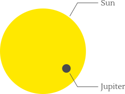
By the same logic, from here on Earth we should be able to detect large planets in other star systems by observing a periodic dimming of the host star. And 1% does not seem to be an exceedingly small number. So can it be done?
I attempted to observe this effect on a star system 64.5 light-years away from us, using a small telescope and a Nikon camera on the balcony of my apartment in Prague. This page describes the result, as well as some of the things I took into account.
A brief history of the observation of planets
We can see Mercury, Venus, Mars, Jupiter and Saturn with the naked eye, so these five planets are well known for millennia. They look different from the Moon and the Sun which appear as disks (not points), and they are also unlike stars whose position in the sky does not change significantly. (The fastest moving star is Barnard's Star which is not visible with the naked eye; its shift in the sky over 170 years is comparable to the size of the Moon.)
And then came the telescope. Using one, William Herschel spotted a 'nebulous star or perhaps a comet' in 1781. It moved over time, and this motion was found to correspond to an approximately circular orbit around the Sun. It had no coma or tail (unlike normal comets). And under large magnifications this object seemed to increase in size (unlike actual stars). And so it was quickly made clear that for the first time since antiquity a new planet was discovered: Uranus.
Several decades later (1846), in a famous episode of the history of astronomy, Urbain Le Verrier predicted
Neptune's existence as well as its expected position, which was immediately confirmed by Johann Galle at the
Berlin Observatory. Then, in 1930 it was Pluto's turn to be discovered, although in 2006 the International
Astronomical Union defined a planet in such a way that it excludes Pluto. This dwarf planet (as it is now
classified) is very dim, but still it can be imaged from an apartment in a major city
 .
.
The hunt for other planets in the Solar system is ongoing. Two very important parameters are the mass and distance to the Sun of these hypothetical bodies. It seems that right now we cannot rule out the existence of a planet as massive as Saturn if it were around 1000 astronomical units (AU) away from us (1 AU is the average Earth-Sun distance, which is about 150 million km). A new planet the size of the Earth could be lurking as close as 200 AU from the Sun, which is just about 5 times the average distance to Pluto. At least that is the conclusion of this paper (figure 5 in particular). What are the main experimental constraints?
- Perturbations on the orbits of the known astronomical bodies (such as the planets) must be small, since their orbits have been measured with great precision. For example, the position of Saturn seems to be well understood up to 100 meters or so.
- A planet orbiting the Sun at a very large distance (more than ~1000 AU) would have been stripped from the Solar System by gravitational interactions with nearby stars. After all, over millions of years the relative position of stars changes appreciably, and therefore the Sun surely had many close encounters with other stars. This consideration is particularly important immediately after the creation of the Solar System in a star cluster, where the average distance between stars was small.
- The Wide-field Infrared Survey Explorer (WISE) — a space telescope — has not seen seen bodies like Saturn and Jupiter closer than 28000 and 82000 AU, respectively. Why is infrared radiation important? Sunlight reaching a planet at a large distance $d$ drops as $1/d^2$ so the reflected sunlight reaching us from such body drops as $1/d^4$. The advantage of looking for infrared radiation is that, provided that the planet's main heat source is not the Sun, then we can expect only a $1/d^2$ drop-off from its infrared light.
Exoplanets
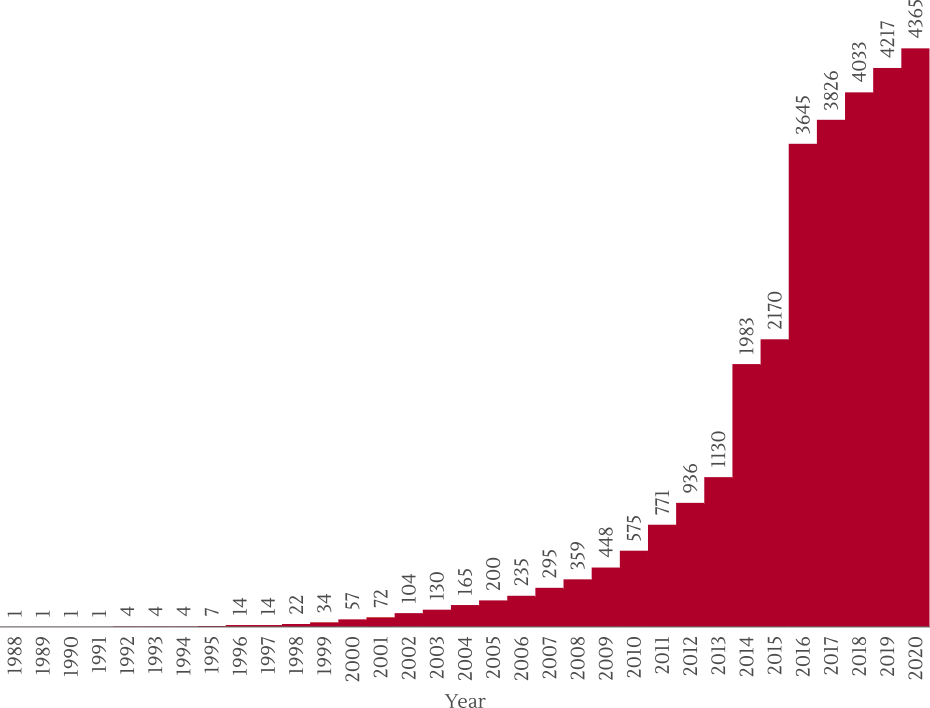
By the late 1980's some evidence started to appear that other stars also have planets. This was confirmed in the 1990's and since then thousands of planets outside the Solar System (exoplanets) have been discovered. The following graphs shows the evolution with time of the cumulative number of known exoplanets (according to the Exoplanet Encyclopaedia):
They have been detected with a variety of methods. The transit method mentioned at the very start of this text is likely the only one which can also be used by amateurs from home. The main point is that if the exoplanet comes in between us and its host star, we will see a dimming of that star.
But can we do that from an apartment's balcony? It seems discouraging that professional astronomers have only convincingly identified exoplanets in the last 30 years; nevertheless it is worth trying.
The equipment I used was the William Optics 6.1cm aperture telescope which is not much bigger than a half-liter Coca-Cola bottle
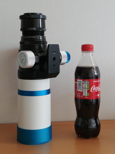
plus a Nikon D5300 camera and a tripod. To track the sky and avoid star trails, I used the Sky-Watcher Star Adventurer. However, this last equipment might not be crucial for this experiment. Also, I used a filter to remove some of Prague's light pollution, although this turns out not to be important either.
Finding a good target
Two factors must be taken into account when picking an exoplanet to observe.
- The planet's orbital plane must be aligned with the Earth, so that we see the planet transiting over the star.
- The Earth is essentially a big spinning top, which means that there are parts of the sky in every location (except the equator) that are never visible. This is particularly significant at high latitudes, as we get closer to the Earth's poles. Prague is 50º North of the equator, so in the following I will consider only exoplanets which rise at least 10º above the horizon here. In the equatorial celestial coordinate system, this means that only targets with a declination of -30º or higher will be considered.
The list of exoplanets which meet these two criteria were extracted from the Exoplanet Encyclopaedia. Two extra properties to consider is the brightness of the host star, as well as the transit depth which consists of the fraction of starlight obstructed whenever there is a transit. Here is a plot of these two quantities for the possible targets:
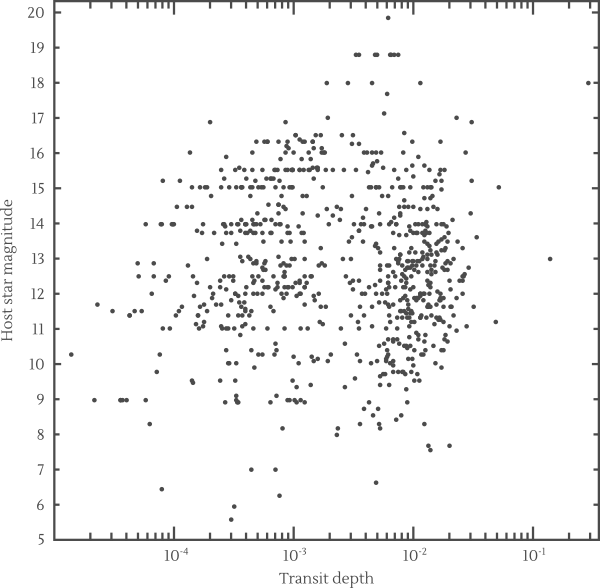
From my experience, stars fainter than magnitude 13 can be spotted, but observing variations of their brightness against a light polluted sky is difficult (except perhaps for very large variations). On the other hand, even if the host star is very bright, exoplanets which only dim it by a $10^{-3}$ faction (a one per thousand factor) are likely beyond what one can hope to detect with simple equipment. These considerations significantly reduce the list of potentially interesting exoplanets.
What should be prioritized? A brighter host star or a larger transit depth? I'm not sure. Under the wrong but hopefully not too wrong assumption that most of the noise in the final results will be due to a statistical fluctuation of the measured starlight (shot noise) then, in order to maximize the signal to noise ratio we would need to maximize $f \sqrt l$ where $f$ is the transit depth and $l \propto 100^{-m/5}$ is the host star brightness ($m$ being its apparent magnitude). So I have drawn lines of constant $f \times 100^{-m/10}$ below.
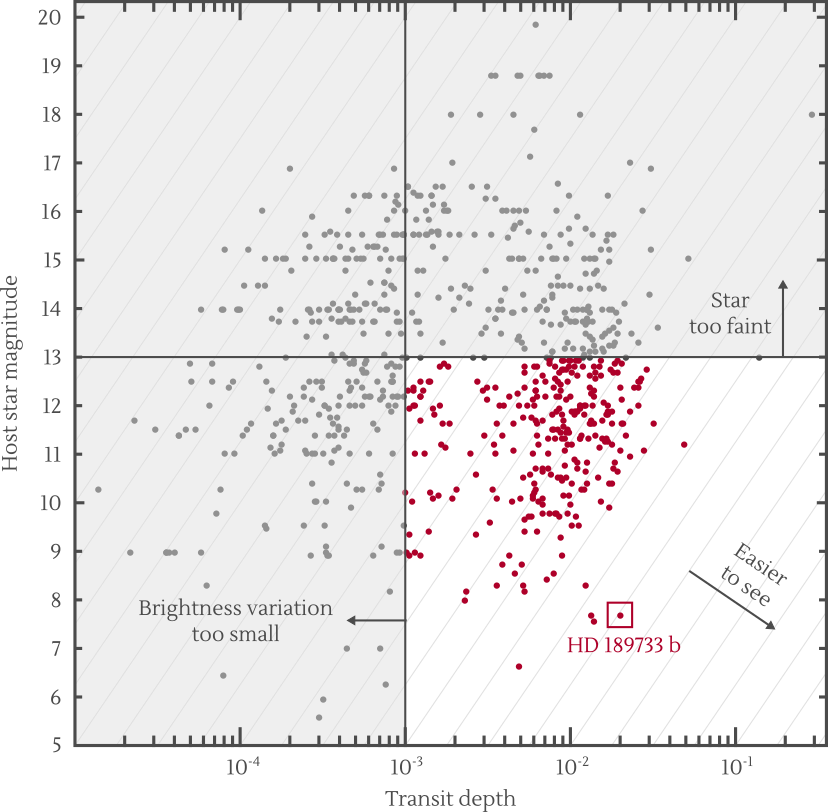
Under this criteria, HD 189733 b is the easiest exoplanet to see, although there are a few other potentially interesting targets.
HD 189733 b
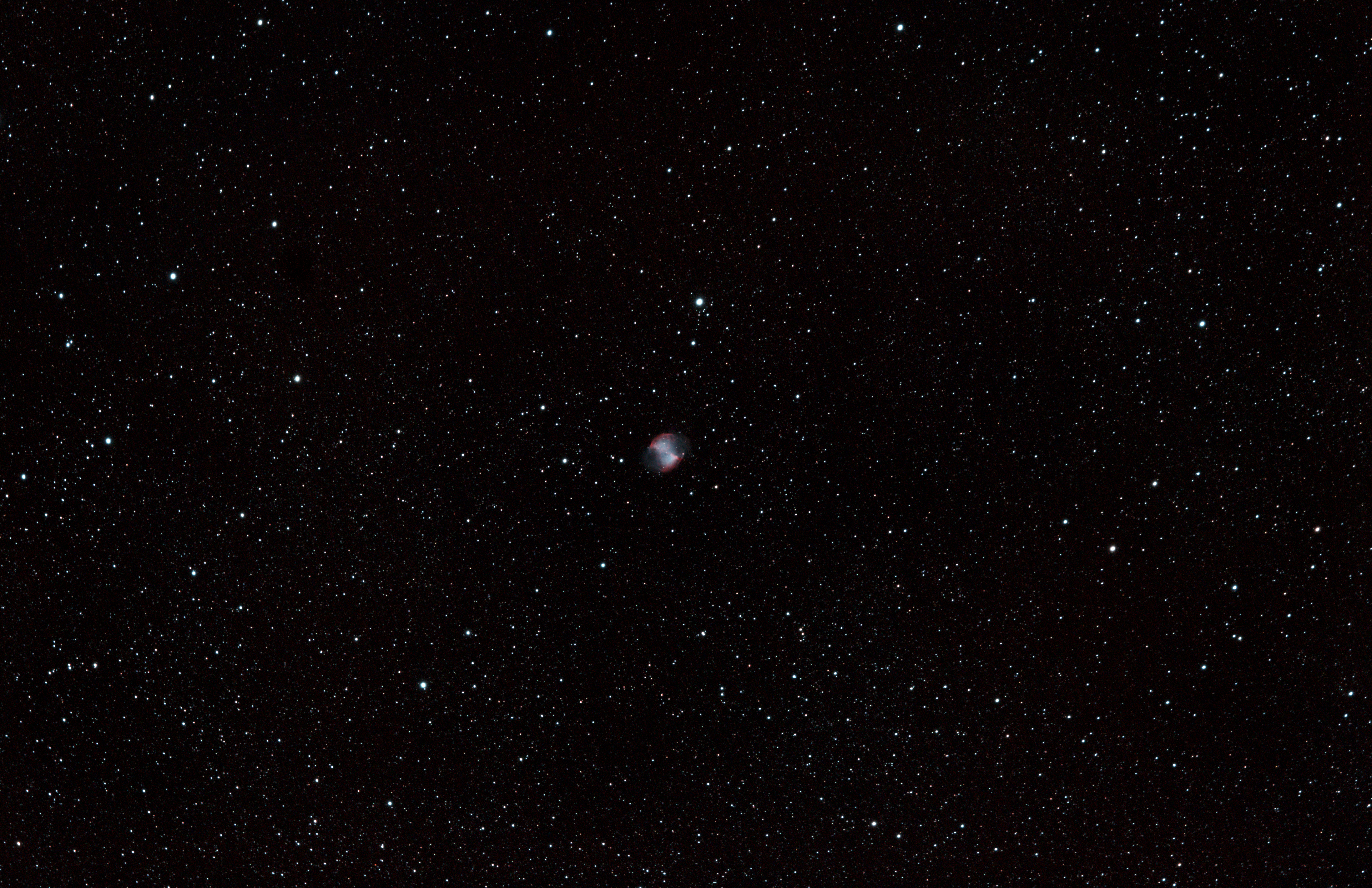
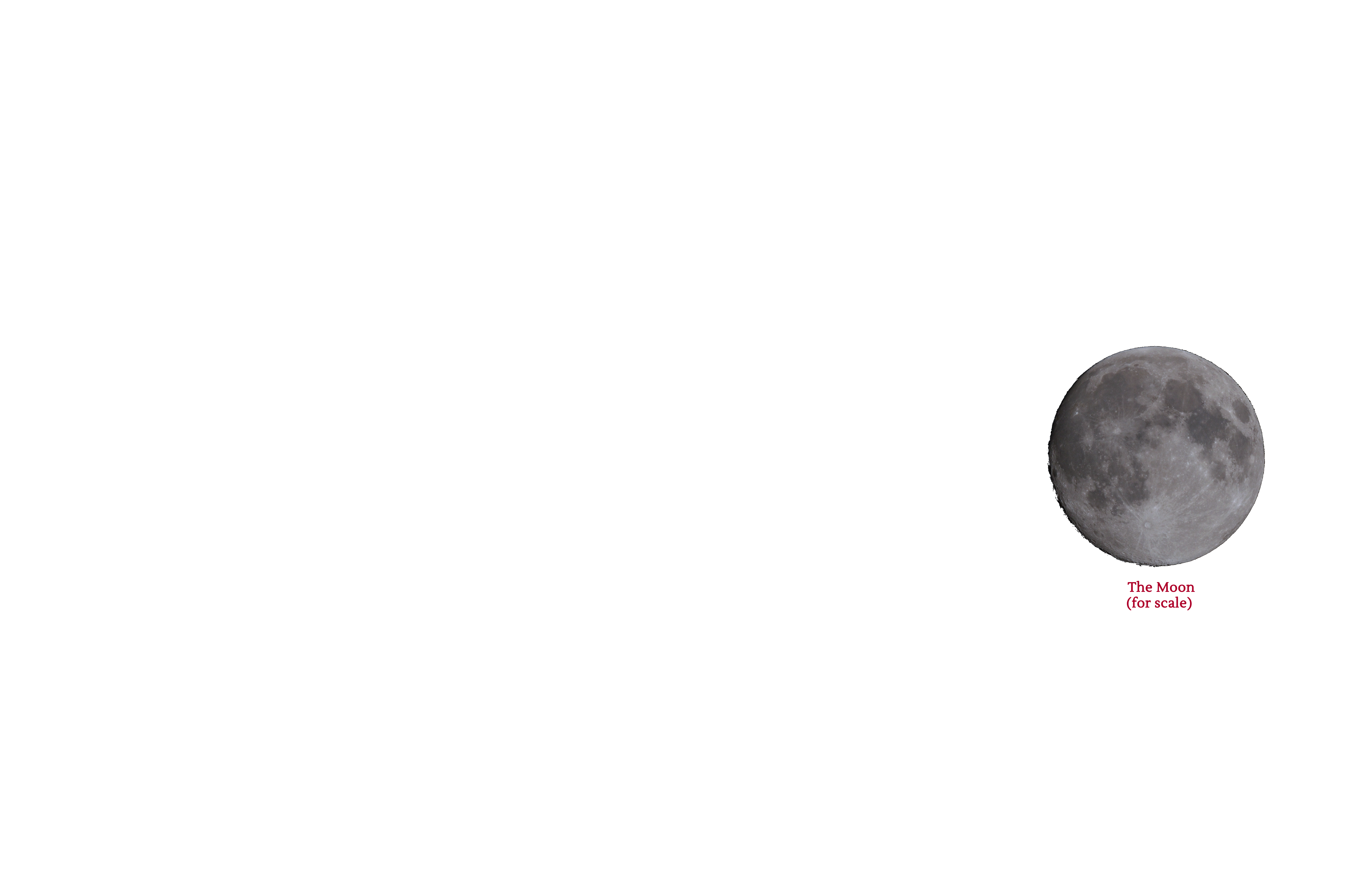
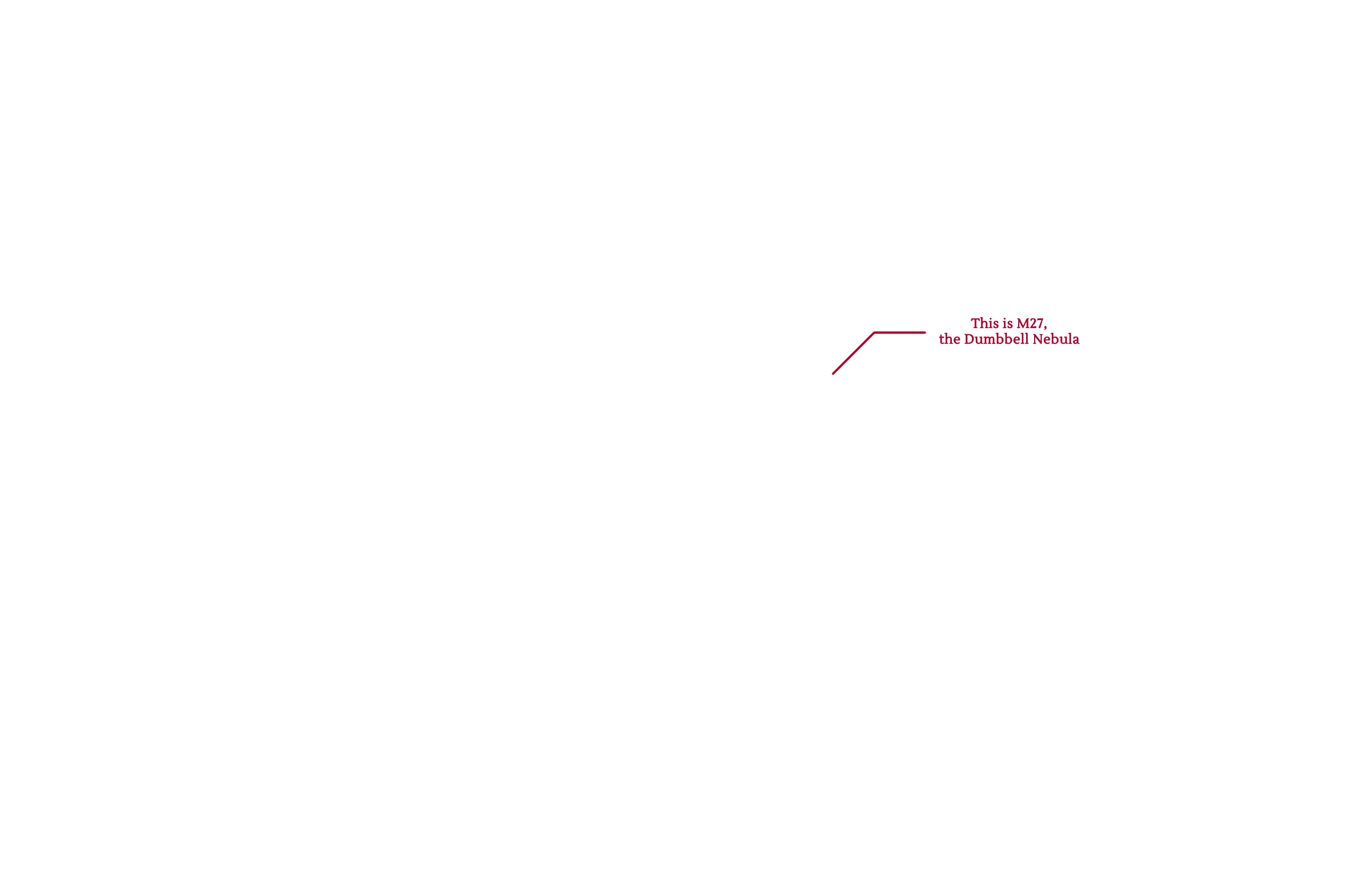
First up, we need to locate this object, which orbits a star with the same name but no 'b'. So where in the night sky can we find HD 189733? Amazingly, this star is very close to a well known deep sky object called the dumbbell nebula which was discovered in 1764 by Charles Messier and later included as the 27th object (M27) in the now famous Messier catalogue of nebulae and star clusters.
Here is an image of M27 that I obtained by combining several photos taken on the 21th of September 2020, together with the location of HD 189733:
Here is why we should care about the 'control 1' and 'control 2' stars. The measured brightness of HD 189733 may change for a variety of reasons unrelated to exoplanet transits (passing clouds, for example). That is why we need the stars 'control 1' and 'control 2': they are close to our target HD 189733, and they have a similar brightness so we can use them to factor out the effects of uncontrollable atmospheric conditions. In practice this can be done by tracking the ratio 'brightness of HD 189733'/'brightness of control 1 or 2'.
Collecting data
The plan is to take many photos of HD 189733 over time, so we must now consider what to do, in practice, to measure a star's brightness from a photo. One idea is to draw a square covering the star, count the RGB values of each pixel inside it, and then sum everything. This is a good strategy, but for best results it is important to make some refinements. The first problem is light pollution: not all light coming from the square is starlight, so we must estimate the amount of light pollution in a particular portion of the sky at a given time. How can we estimate this unwanted background light? One possibility is to compute the brightness of the sky in empty patches around our star, like this:
![]()
The four rectangles I used have the same total area as the central square, so a good estimate of a star's brightness is to count the total value of the pixels in the square minus those in the four rectangles.
Another thing to note is that a camera's sensor does not measure color, which is related to the frequency of photons. Rather, the sensor only counts photons. So the trick used by manufactures to capture color images is to cover each pixel with a red, green or blue filter, usually in a repeating 2x2 pattern. This is called a Bayer filter. In this way each pixel becomes sensitive only to one of these three colors. The camera measures one value for each pixel (corresponding to the intensity of red, green or blue light) and not three, but software then interpolates this information to produce RGB values for all pixels. Ideally, one should then use the raw data captured by the camera rather than post-processed one.
The linearity of each pixel's signal with the amount of photons hitting it might also be important. Imagine that due to atmospheric turbulence or camera shaking in some photos a star becomes blurry and covers twice as many pixels as in other photos. The number of photons hitting each pixel drops to half, but if the signal registered in each pixel does not decrease to half we would have a problem. So it is important to understand how the signal varies with the number of photons hitting a pixel in order to correct for any non-linearity.
I did so for my D5300 Nikon camera. One can for example take a series of photos in a controlled environment with different exposure times (1/10s, 1/5s, 1/2s, 1s, ...) which should be proportional to the number of photons, and check how does the signal produced changes. The sensor response function was analyzed in this way, and this information was then used to correct the value of each pixel to a linear scale when imaging the sky.
With this said, I took 606 photos of HD 189733 (and the surrounding patch of sky) on the 7th of September 2020 from the balcony of my apartment. Each photo had an exposure of 20 seconds, and they were made one right after another, except for some pauses lasting a few minutes to reposition the telescope. Here is how the stars looks in each frame:


You may have noticed some things:
- The stars are bluish. This is because I used a filter over the camera sensor to cut some of the light pollution typical of a big city. Yellow and red colors are suppressed, hence the blue tone of the three stars. Nevertheless, it seems to me that usage of such filters is unnecessary for this experiment.
- The stars are defocused, appearing as blobs which are quite large. That is intentional — the idea is to spread each star's light over an extended area in order not to saturate the sensor pixels. If this were to happen, some of the light hitting the sensor would not be registered.
- In some frames, the stars seem to suddenly become more defocused/fuzzy. This might be due to changing atmospheric conditions.
- With a sharp eye, in some frames one can see dots moving close to the stars. These are hot pixels of the sensor, which are at fixed positions; it is actually the stars that move a bit from frame to frame across the camera's sensor. These hot pixels are a source of error (which is not sizable), as they are included in the measurement of a star's brightness (or in the background luminosity estimates).
With all this said, here is a plot with the brightness of HD 189733 and the two control stars:

The horizontal axis represents the photo number (1 to 606), and since there were some brief pauses in the photo-taking process, it is not a faithful representation of time. In a moment, I will correct for this using the time of each photo as recorded by the camera.
On the other hand, the vertical axis represents brightness in some scale whose units are irrelevant. But crucially this is a linear scale of brightness. The process of extracting data from each photo was done automatically with a small computer program.
The signal+background values correspond to the central squares I mentioned earlier, while background (in gray) refers to the brightness of the rectangles around the central squares. The signal data is just the difference between the two. It is noticeable that the background brightness increases over time, while the signals goes down. I think this is due to the fact that the altitude above the horizon of the patch of the sky under observation decreased over time, which would explain the increasing background, due to more light pollution. Starlight should also be absorbed more by the atmosphere given that it has to travel through an increasing amount of air before reaching the telescope, thereby explaining the decreasing signal.
Note also the large brightness variation of all three stars: for example HD 189733's signal seems to vary from around 120.000 to 100.000, a 20% difference! The change of brightness we want to measure due to an exoplanet transit is just around 2%, so this would be a problem. That is the reason why the control stars are important: in the end, we can control for atmospheric effects by looking at the ratio of star brightnesses.
But before performing these ratios, let us discuss the timing of the transits of HD 189733 b.
When to expect a transit?
It is not possible to observe 24 hours a day this patch of the sky and wait for a transit, since at the very least there is the problem of daytime. In fact, due to other constraints (the orientation of my apartment and not being able to image parts of the sky too high in the horizon which are obstructed by the ceiling), I can only image HD 189733 for perhaps 4 hours a day.
It is therefore desirable to known beforehand when do transits occur. According to the paper Eric Agol et al 2010 ApJ 721 1861 a transit (the middle of it) occurred on 2454279.436714 BJD, and the recurrence period of these events is 2.21857567 days. BJD is a reference to barycentric Julian date. If we forget the "B" then a Julian date (JD) is given by the time elapsed since 12:00 (GMT timezone) 24 November 4714 BC, measured in days and fractions of a day. For example, the start of the year 2021 in the GMT+1 time zone corresponds to 2459215.4583 JD.
The problem with Julian dates in astronomy is that the Earth moves around the Sun. If the Earth was right between the Sun and some object under study (such as HD 189733), light from this source would reach us around 16-17 minutes earlier than if the Earth was behind the Sun. This means that the transits of HD 189733 b are slightly irregular in JD time since the Earth will move back and forth from the star over each year. The problem is solved with barycentric Julian time, which uses the Sun as a reference point. So BJD and JD will differ at most by around 8 minutes, which is not much, but as we will see it is worth accounting for this difference.
So in practice how can one get BJD from JD? All we need is the angle $\theta$ between the Sun and the star under consideration:

Since in most cases the Sun-Earth distance $r$ is much smaller than the Earth-star distance $d^\prime$ the approximation $d^\prime-d=r \cos \theta$ is excellent. The time taken by light to cover this distance accounts for the effect we are discussing. Using $r/c\approx500\textrm{ s}$, \[ BJD-JD\approx500\cos\theta\textrm{ seconds} \]
Looking at a sky chart, the angular separation between the Sun and HD 189733 was about 126.5º which implies that $BJD-JD\approx -4.92$ minutes, that is the starlight was reaching Earth almost 5 minutes before it would reach the Sun. (For night observations we do expect this number to be negative, as the Sun tends to be in our back when we are facing the night sky.)
Here is a table with the a list of 10 recent and future transits, computed with a small script which uses your computer clock:
| Date and time of past and future transits |
|---|
These times refer to the center of the transits (each event lasts 1h 49m according to the reference mentioned earlier).
Results
This means that HD 189733 b was halfway through a transit at 23:28:30 GMT+2 of 7th September 2020. The plot shown earlier with the brightness of the stars HD 189733, control 1 and control 2 captured the entirety of this transit. And now, instead of providing the data for photo 1, 2, ..., 606 we can plot the stars' brightness over time, with time=0 corresponding to the predicted center of the transit. After subtracting the background luminosity for each star, and performing the ratio of star brightnesses described earlier, here is what I got.


Although the data fluctuates significantly from photo to photo, just looking by eye it does seem that from for a period of around 2 hours the brightness of HD 189733 decreased by a few percent!
We can now compare with data from the paper Eric Agol et al 2010 ApJ 721 1861, which used the Spitzer space telescope (it sees in the infrared). Furthermore, we may also try to fit some curves to the above points. In order to do so without thinking too much, we may do as follows. The light-curve of HD 189733 during a transit can be extracted from the Spitzer paper; let us call it $\mathcal{S}(t)$ where $t$ is time. Besides comparing $\mathcal{S}(t)$ to the data above, we can also deform its shape to $\mathcal{S}\left(h,\varepsilon_{f},s,\varepsilon_{T},t\right)$ such that we can change and fit the transit depth $\varepsilon_{f}$, the time-shift $s$ of the transit from its known value, and the transit duration $\varepsilon_{T}$:
\[\mathcal{S}\left(h,d,s,\varepsilon_{T},t\right)=h\left[1-\varepsilon_{f}+\varepsilon_{f}\mathcal{S}\left(t/\varepsilon_{T}-s\right)\right]\]The $h$ variable is a normalization: it measures the ratio of the star brightnesses (HD 189733/control 1 or 2) and therefore it is not described in the Spitzer paper. Note also that the quantity $\varepsilon_{f}$ measures the percentage of light obstructed by the planet during a transit relative to the number predicted using Spitzer (which is 0.0241). So the fraction of light blocked is $f=\varepsilon_{f}f_{\textrm{Spitzer}}$ with $f_{\textrm{Spitzer}}=0.0241$. The same is true for $\varepsilon_{T}$ which measured the transit duration relative to the one obtained by professional astronomers ($T_{\textrm{Spitzer}}=1.824$ hours).

With this said, we can try to infer these 4 parameters ($h$, $\varepsilon_{f}$, $s$ and $\varepsilon_{T}$) from the data by doing fits. To do so, we must estimate the error association to each measurement of the ratio of star brightnesses. I came up with the following numbers, which seem sensible. We may use the standard deviation of the data itself to estimate errors, however since we have a transit, this error should be taken from the ratio of brightnesses of the two control stars and then scaled appropriately to take into account the mean values of 'HD 189733/control 1' and 'HD 189733/control 2'. In the end, for each value of 'HD 189733/control 1' I assumed an error of 0.023 and 'HD 189733/control 2' the value used was 0.017. These two numbers are similar in size to the transit depth which we seek to observe, but given that there are hundreds of data points, that it still good enough to (a) observe without a doubt the effect of the transit and (b) extract some interesting data about it (as we shall see now).
One can also evaluate the likelihood of an hypothesis being true from the data. For example, how likely is it that there was no planet transit at all, and that we are just seeing noise? An hypothesis excluded or in tension with the data at N$\sigma$ is an unlikely one for N above 3 since the chance of it being true is smaller than 0.27%; if N is above 5 this chance drops to 0.00006% and for N above 10 it is less than 0.000000000000000000002%. We shall see that the 'no transit' hypothesis is even less likely than this!
Using control star 1, these are the best fit values:
| Parameter | Best fit value | $2\sigma$ interval | True value (from Spitzer) |
|---|---|---|---|
| $h$ (normalization) | 1.4879 | 1.4854 to 1.4902 | — |
| $\varepsilon_{f}$ (transit depth) | 0.89 | 0.76 to 1.01 | 1 |
| $s$ (time shift) | -1.2 min | -3.9 to 1.8 min | 0 min |
| $\varepsilon_{T}$ (transit duration) | 0.92 | 0.85 to 0.98 | 1 |
Not only can the transit be seen, but the precision on some of its parameters is actually quite good. For example, the middle of the transit can be determined to a few minutes (this vindicates the extra effort in dealing with barycentric Julian dates).
One might wonder if this precision is not an artificial consequence of considering an excessively small error for each data point (0.023). This does not seem to be the case, and in fact the error might be a bit conservative. That's because the quantity $\chi^2/N$ (chi-squared per data point) which measures the quality of the fit is only 0.30 (significantly smaller than 1).
There are two other important numbers: the hypothesis of there being no transit can be excluded at 14.2 $\sigma$ ($\Delta\chi^2\approx 211$; 3 degrees of freedom) and furthermore there is a 3.0 $\sigma$ tension with the Spitzer data ($\Delta\chi^2\approx 13.8$; 3 degrees of freedom). This tension is sizable but still not very concerning.
The data points, the Spitzer data and the best fit curve look like this:

All this analysis can be repeated using control star 2. The best fit values are as follows:
| Parameter | Best fit value | $2\sigma$ interval | True value (from Spitzer) |
|---|---|---|---|
| $h$ (normalization) | 1.1255 | 1.1235 to 1.1273 | — |
| $\varepsilon_{f}$ (transit depth) | 1.06 | 0.94 to 1.18 | 1 |
| $s$ (time shift) | -2.0 min | -4.6 to 0.8 min | 0 min |
| $\varepsilon_{T}$ (transit duration) | 1.04 | 0.96 to 1.12 | 1 |
The no transit hypothesis is excluded at 17.6 $\sigma$, and the data is compatible with the one of Spitzer at 1.0 $\sigma$.

This leaves me in no doubt that exoplanet transits can indeed be spotted from a balcony in a big city, with a small telescope and a DSLR camera. It is great that the star dimming associated to a transit is observable!
We might as well conclude the discussion here, but the remarkable precision with which some of the transit parameters can be estimated should motivate us to look at the data a bit more carefully.
Thinking about the geometry of the problem
The parameters estimated above ($h$, $\varepsilon_{f}$, $s$ and $\varepsilon_{T}$) just measure deformations of the light curve obtained with Spitzer. I did this in order not to have to think about how such curve should look like from the physical characteristics of the star-planet system (the size of the planet and the star, the orbit radius, and so on). However, maybe it is worth doing that after all. So, can we learn something about the HD 189733 planetary system?
Although we cannot resolve its features, what we are observing is probably something like this:
The variation with time of the star's brightness should depend on several parameters (I will assume that the planet's orbit is circular):
- The ratio of the planet's radius $r$ to the star's radius $R$. In fact, the faction of light blocked during a transit should be close to $(r/R)^2$ (more on this later).
- The period $P$ of orbital rotation of the planet. If we manage to measure any dimming of the star at all, this parameter should be straightforward to estimate since it is the recurrence time of these events.
- The timing $t_0$ of a transit center, when the planet is half-way through the transit. Other transit centers occur at the times $t_0 + P$, $t_0 + 2P$, etc.
- The distance $d$ of the planet to the star. The percentage of time that the planet is blocking the star depends on this number or, more specifically, on the ration $d/R$. Just consider that in the limit where the planet is constantly grazing the star's surface ($d=R$), the planet is blocking the star's light half of the time, while for larger (and more reasonable) distances $d$ this percentage decreases.
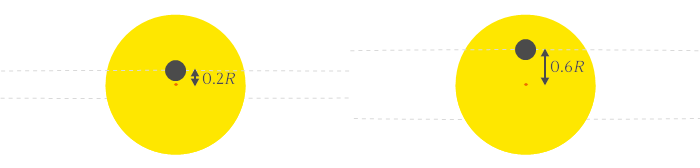
- We are unlikely to be viewing the planet's orbital plane exactly edge on, so what is called the impact parameter $b$ is an important variable. We may define this number in such a way that $B \equiv b R$ is the closest apparent distance (as seen from our vantage point) that the center of the planet comes to the center of the star. Here are two drawings showing the situation for $b=0.2$ and $b=0.6$.
Note that nothing above depends on the absolute size of the star system, as we can only measure ratio of distances: $r/R$, $d/R$ and $b=B/R$. So we will never be able to use purely geometric considerations to distinguish a star with a radius of 1 million km from one with a radius of 1 mm (!).
Here are two animations showing the light curves for different impact parameters. On would expect that a fraction of light $(r/R)^2$ is blocked in the middle of a transit, however if the planet only grazes the star ($b$ must be close to 1) then this fraction can be smaller, as shown in the second animation.
Now let us do some math. We need two formulas: one for the overlap of two circles with radius $r$ and $R$ whose centers are a distance $\Delta$ apart, and then we must compute this separation $\Delta$ as time $t$ evolves. The answer to the first problem is
$$\begin{align*} \textrm{Overlap}\left(r,R,\Delta\right)= & r^{2}\arccos\left(\frac{\Delta^{2}+r^{2}-R^{2}}{2\Delta r}\right)+R^{2}\arccos\left(\frac{\Delta^{2}-r^{2}+R^{2}}{2\Delta R}\right)\\ & -\frac{1}{2}\sqrt{(\Delta+r-R)(\Delta-r+R)(+r+R-\Delta)(\Delta+r+R)} \end{align*}$$
A small detail: assuming that $r$ is smaller than $R$ we see that this formula is problematic when the distance $\Delta$ is outside the interval [$R-r$,$R+r$] (because we are forced to calculate the arc cosine of a number either smaller than -1 or larger than 1). However, the real result for that case is clear: there is no overlap between the two circles if $\Delta>R+r$, and for $\Delta \leq R-r$ the overlap is maximal — i.e. $\pi r^2$. (This minor nuisance can also be neatly solved by taking the real part of the formula above; that result will be valid for any value of $\Delta$.)
Anyway, this a purely mathematical result related to two circles and by itself has nothing to do with planets and stars. Now, to find $\Delta$ as time changes we need to consider the orbit of a planet around a star as seen from very far away.
I will assume that the orbit is circular, with radius $d$. Because of the angle of this orbit with our line of sight we will see the planet describing a squashed circle — an ellipse to be more precise. On the un-squashed axis, the planet appears to reach a maximum separation $d$ from the star, but on the other one this distance is reduced to $b R$ where $b$ is the impact parameter mentioned earlier.

From this observation, we may readily conclude that the distance $\Delta$ between the star and the planet (as seen from Earth) is given by the formula \[ \Delta\left(t,b,d,P,t_0\right)=\sqrt{\left(d\sin\frac{2\pi (t-t_0)}{P}\right)^{2}+\left(b R\cos\frac{2\pi (t-t_0)}{P}\right)^{2}} \] where $P$ is the orbital period.
In conclusion, the fraction of the star covered by the planet at any given time $t$ is then given by the expression
\[ \frac{\textrm{Re}\left[\textrm{Overlap}\left(r,R,\Delta\left(t,b,d,P,t_0\right)\right)\right]}{\pi R^{2}} \]As states earlier, this result cannot depend on the absolute scale of the star system, and indeed it can be check that this formula is equal to
\[ \frac{\textrm{Re}\left[\textrm{Overlap}\left(r/R,1,\Delta\left(t, b,d/R,P,t_0\right)\right)\right]}{\pi} \]We can then go ahead and see what the data is telling us about $b$, $d/R$, $r/R$, $P$ and $t_0$.
Estimates for the planetary system HD 189733
Transit centers can be determined with an accuracy of a few minutes, so by waiting enough time one can determine with very high precision the orbital period $P$. For example, in a year the planet will complete more than a hundred revolutions over the host star, so from two transit observations an year apart (and assuming we do know the exact number of transits which occurred in between) one can determine $P$ with an error of the order of a second.
That is why in the following I will assume that $P$ is known to be equal to 2.21857567 days (the Spitzer value). We are left with 4 quantities to determine: $d/R$ (the orbital radius compared to the star's radius), $r/R$ (the planet's radius compared to the Star's radius), $b$ (the impact parameter) and $t_0$ (the transit center time compared to the prediction from Spitzer). Here are the results, using each of the control stars:
| Parameter | Best fit value | $2\sigma$ interval | True value (from Spitzer) |
|---|---|---|---|
| $r/R$ (planet size) | 0.143 | 0.133 to 0.154 | 0.155313 ± 0.000188 |
| $d/R$ (orbit radius) | 12.3 | 9.2 to 13.4 | 8.863 ± 0.20 |
| $b$ (impact parameter) | 0.47 | 0 to 0.78 | 0.6631 ± 0.0023 |
| $t_0$ (time shift) | -0.1 min | -2.2 to 2.9 min | 0 min |
| Parameter | Best fit value | $2\sigma$ interval | True value (from Spitzer) |
|---|---|---|---|
| $r/R$ (planet size) | 0.159 | 0.150 to 0.173 | 0.155313 ± 0.000188 |
| $d/R$ (orbit radius) | 7.6 | 5.3 to 11.5 | 8.863 ± 0.20 |
| $b$ (impact parameter) | 0.79 | 0.45 to 1.12 | 0.6631 ± 0.0023 |
| $t_0$ (time shift) | -2.1 min | -5.2 to 1.1 min | 0 min |
It is interesting how it is possible to extract this information about a star system dozens of light years away, with only a small telescope in the middle of a city. As one can see, these results are in reasonable agreement with Spitzer data, and the precision is not so bad either. However, it is worth noting that the numbers for $r/R$ and $t_0$ are substantially more precise than those for $d/R$ and the impact parameter $b$.
Why is that? Well, changes of $r/R$ leave a clear mark on the light-curve because this parameter controls de transit depth, which is the fraction of light blocked. Likewise the $t_0$ parameter can be straightforwardly estimated from a light-curve.
On the other hand, things are not so simple for $d/R$ and $b$. For all other parameters fixed (including the orbital period $P$), if we increase the orbit size $d$, the fraction of time the planet is blocking starlight decreases; in other words, the transit time decreases. This would then be a parameter easy to determine, if it were not for the fact that increasing $b$ has a similar effect. Indeed, as the planet transits the star further from its center (larger $b$), the transit time also decreases. So it is hard to disentangle these two parameters: the effect of a larger (smaller) $d/R$ can be, for the most, compensated with a smaller (larger) $b$. This compensation is not perfect and that is why it is possible to have an estimate for these two quantities.
One can better appreciate this matter by plotting the 2-dimensional best-fit regions for $d/R$ and $b$:

The existence of a long band of values in this $d/R$ versus $b$ space which fits well the data is due to effect just discussed. As a side note, I'll mention that in principle $b$ can be larger than 1, however in those cases the transit depth will decrease considerably unless the size of the planet $r/R$ (not shown in this plot) is also increased.
A final consideration: limb darkening
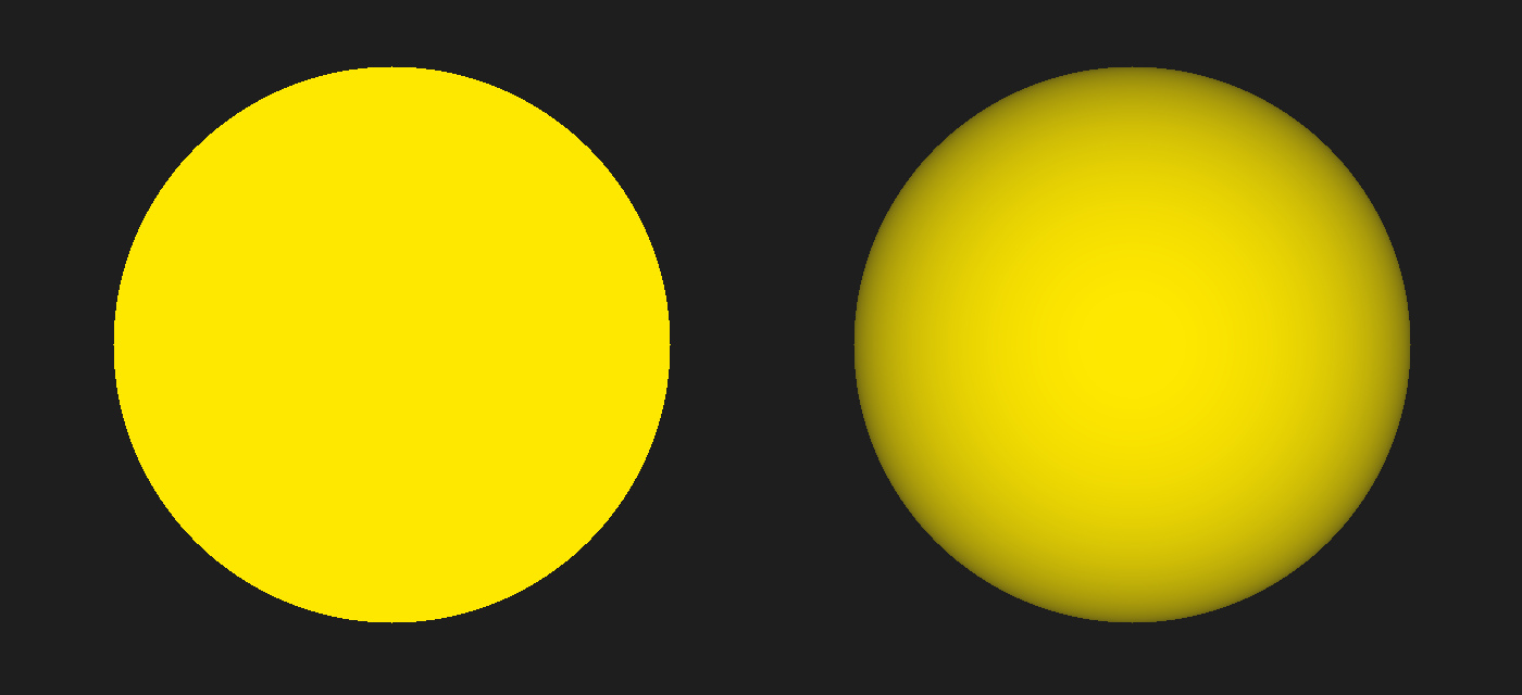
A potentially important effect which was not taken into account so far is the limb darkening of the disc of a star. The previous results assumed that a star has uniform brightness. However, in reality it is known that the center is brighter, with the luminosity falling off as we approach the edge of the disk. In the computer generated image below, on the left there is a disk with no limb-darkening and on the right there is a realistic depiction of what happens with the Sun:
The dependence of the brightness $I$ (per unit of surface) on distance to the center of a star's disk (we may use the impact parameter $b$ to measure this distance) appears to be well approximated by the expression
\[I(b)=I(0)\left[1+A_{1}\left(1-\sqrt{1-b^{2}}\right)+A_{2}\left(1-\sqrt{1-b^{2}}\right)^{2}\right]\]The numbers $A_1$ and $A_2$ depend on each star. In the case of the Sun, $A_1=-0.47$ and $A_2=-0.23$ seem to be adequate, so these are the numbers I used to produce the image above.
The analysis of the transit of HD 189733 b can be redone taking into account this effect, instead of a disk with uniform brightness ($A_1=A_2=0$). Ideally, one would leave $A_1$ and $A_2$ as free parameters and fit them, which is to say that these numbers would also be inferred from the data. That seems to be what the authors of Eric Agol et al 2010 ApJ 721 1861 did using the Spitzer space telescope (for $A_1$ only; $A_2$ was assumed to be 0). But it seems to me that in order for this to be a valid strategy, one would need to have high precision data, which is not my case. Therefore, I repeated the analysis shown above assuming that HD 189733 is a star with limb darkening similar to the one of the Sun: $A_1=-0.47$ and $A_2=-0.23$.
It is now harder to obtain nice looking mathematical expressions for the expected light curve as a function of the star system properties. Nonetheless, one can still numerically find the best fit values for the various parameters. The results are as follows (best fit values and 2$\sigma$ intervals). Using control star 1: $r/R=$ 0.135 (0.125 to 0.147), $d/R=$ 11.8 (9.7 to 12.7), $b=$ 0 (0 to 0.70) and $t_0=$ 0 minutes (-2.0 to 3.4 minutes). Using control star 2: $r/R=$ 0.150 (0.139 to 0.171), $d/R=$ 10.2 (6.4 to 11.3), $b=$ 0.64 (0 to 0.85) and $t_0=$ -2.4 minutes (-5.3 to 0.9 minutes).
Notice how the estimates for the radius of the planet are somewhat smaller with limb darkening taken into account. That is because the average brightness of the Sun's surface is only 80.5% of the brightness at its center. Therefore, a planet with $r/R=0.1$ (for example) passing through the center of the star's disk would lead to a 0.0124 decrease of its luminosity (a larger number than the naive expectation $(r/R)^2=0.01$). So smaller planets can block more light when limb darkening is considered.
The reason I do not highlight too much the results above is because HD 189733 seems to be a star with a rather weak limb darkening. Indeed, the Spitzer study found that $A_1=0.118$ and it assumed that the $A_2=0$. This means that the appearance of HD 189733 is much closer to a uniform disk than to the Sun.
Conclusion
With all this, I would say that it is definitely possible to observe an exoplanet, from home, as it passes periodically between us and its host star. A small telescope (or perhaps a telephoto lens) is enough, and the experiment works even when performed in a large city. With a little bit of patience, one can also extract information on the planetary system, such as the size of the planet and its orbital distance relative to the star's size.
My target was HD 189733 b, which is probably one of the best exoplanets to try to observe. To see or infer the presence of most of the other exoplanets which are now known to exist, one might need much more sophisticated equipment and better observation conditions.
